This project entailed the construction of an interactive visual program where the user can herd flocks of virtual birds known as “boids” — on-screen models which behave as birds in a flock, fish in a school, or mammals in a herd — which follow a simple behavioral model based on what each individual on-screen boid can perceive around them. The intended full model includes alignment with nearby flock mates as well as movement towards and around a target in the user’s hand.
Updating a singular boid’s position requires the normalization of several vectors, which presents the need to develop a resource-efficient and low-latency module for vector normalizations. To acquire the three-dimensional position of the target, we implemented stereo vision using a pair of FPGAs — each with their own camera — which communicate with each other through the SPI protocol. Using the target’s positional information, we computed the positions of the boids every frame in three dimensions and overlaid them on the camera footage via a double frame buffer.
The double frame buffer also presented a unique challenge since, due to overlaying the boids over the camera feed, there was a limited amount of additional pixels/DRAM requests that could be made every frame, amounting to roughly 25% of the screen’s area.
For this class project, we committed to having multiple boids follow the target, moving every frame and being rendered at their computed positions. To demonstrate proper depth calculation, we modified every boid’s size based on its depth. The implemented boid update module includes only the target-following force; alignment, cohesion, and separation remain future work.
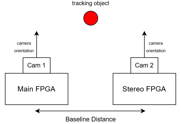
The physical setup: two cameras attached to a pair of Urbana FPGAs.
Contributions
This was a final project for MIT’s 6.2050 Digital Systems Laboratory, built with Sreeja Thipireddy. I was responsible for the implementation of the normalizer, boid manager, and boid update modules. Sreeja was responsible for the implementation of the inter-FPGA communication protocol, depth calculation module, double frame buffer, and modifications to the traffic generator. The renderer module was implemented in collaboration.
Vector Normalization
To compute the necessary vectors in the boid computations, it is necessary to normalize vectors. To normalize a vector, it’s sufficient to multiply the vector’s components by the reciprocal of the vector’s magnitude.
For a vector , we first compute its squared magnitude:
This lets us compute one reciprocal square root and reuse it for all three components.
Initial Approximation
We can compute an initial approximation to the reciprocal of the square root via the position of the number’s most significant bit.
Using , we obtain the initial approximation
For a nonzero integer , the position of its most significant bit is
I implemented a custom combinational module with a tree-based approach which computes the count of leading zeroes. The result for any n-bit number can be derived from the result of its left and right halves. If the upper half of the number contains a 1 bit, the result comes from that half. Otherwise, the result is the width of the upper half plus the leading-zero count of the lower half. This gives us a combinational tree for finding the CLZ. The implementation starts with 32 two-bit pairs: From 00 has two leading zeroes, 01 has one, and a pair starting with 1 has none. Five merge layers combine these counts into the result for the full 64-bit input. In clz_merge, the highest bit indicates that a whole block is zero; the remaining bits encode its leading-zero count.Code: tree-structured leading-zero counter
main/hdl/vec.sv. The source references this leading-zero count tree discussion.module clz_merge #(
parameter WIDTH
) (
input wire [WIDTH-1:0] left,
input wire [WIDTH-1:0] right,
output logic [WIDTH:0] out
);
logic both_full, left_not_full;
assign both_full = left[WIDTH-1] & right[WIDTH-1];
assign left_not_full = left[WIDTH-1] == 1'b0;
logic [WIDTH-2:0] right_chopped;
assign right_chopped = right[WIDTH-2:0];
logic [WIDTH:0] result;
always_comb begin
if(both_full) begin
result = {1'b1, {WIDTH{1'b0}}};
end else if(left_not_full) begin
result = {1'b0, left};
end else begin
result = {2'b01, right_chopped};
end
end
assign out = result;
endmodule
module clz_64 (
input wire [63:0] data,
output logic [6:0] out
);
logic [1:0] bit_pair [31:0];
logic [6:0] assembly_layer [5:0] [31:0];
genvar j;
generate
for (j = 0; j < 32; j++) begin
assign bit_pair[j] = data[2*j+1:2*j];
assign assembly_layer[0][j] =
(bit_pair[j] == 2'b00) ? 6'b000010 :
(bit_pair[j] == 2'b01) ? 6'b000001 :
6'b000000 ;
end
endgenerate
genvar layer, i;
generate
for (layer = 1; layer < 6; layer++) begin
for (i = 0; i < (32 >> (layer - 1)); i += 2) begin
clz_merge #(
.WIDTH(layer + 1)
) m_clz_merge (
.left(assembly_layer[layer - 1][i + 1][layer:0]),
.right(assembly_layer[layer - 1][i][layer:0]),
.out(assembly_layer[layer][i >> 1][layer+1:0])
);
end
end
endgenerate
assign out = assembly_layer[5][0];
endmodule
The squared components of the vector are shifted right by FP_SHIFT before being added, so still has FP_SHIFT fractional bits. If and is the stored squared magnitude, its real value is . The stored reciprocal-square-root estimate therefore needs the scale factor
The code uses e = (3*FP_SHIFT - b) >> 1 for this exponent. It zero-pads the squared magnitude to 64 bits before counting leading zeroes, then uses b = 63 - len_sqr_clz to find its most significant bit. The clocked assignment y_pipe[2] <= (1 << e) << FP_SHIFT gives the estimate an extra FP_SHIFT bits, which are removed by y_pipe_shifted before it is used in the next multiplication.
Code: fixed-point initial estimate
clz_64 m_clz_64 (
        .data({{(64-DOT_PRODUCT_WIDTH){1'b0}},len_sqr_pipe[1]}),
        .out(len_sqr_clz)
    ); // 1

    assign b = 63 - len_sqr_clz; // 1
    assign e = (3*FP_SHIFT - b) >> 1; // 1
Newton-Raphson Refinement
To improve this initial guess, I computed several iterations of a Newton-Raphson approximation scheme. Through a C simulation I found that 4 iterations was enough to achieve visually satisfactory results.
For an estimate of , the iteration is
At the desired value, , so the correction factor is one. Each iteration employs only multiplication and substraction operations. In fixed-point arithmetic, the products also need to be shifted to account for the fractional bits. I split each iteration across three clock cycles: square the current estimate, multiply by the squared magnitude, and apply the correction. THREE_HALFS stores 1.5 in fixed-point format. The expression half_ay2_pipe[i] >> (2 * FP_SHIFT + 1) accounts for the product’s extra fractional bits and divides it by two. The generated stages implement the equivalent form .Code: three-cycle Newton-Raphson iteration
genvar pipe_idx;
    generate
        for(pipe_idx = 3; pipe_idx < 3 + 3*ITERATIONS; pipe_idx += 3) begin
            always_ff @( posedge clk ) begin
                y2_pipe[pipe_idx] <= y_pipe_shifted[pipe_idx-1] * y_pipe_shifted[pipe_idx-1]; // 3*i
                // y2_pipe[pipe_idx+1] <= y2_pipe[pipe_idx];
                // y2_pipe[pipe_idx+2] <= y2_pipe[pipe_idx+1];

                // half_ay2_pipe[pipe_idx] <= half_ay2_pipe[pipe_idx-1];
                half_ay2_pipe[pipe_idx+1] <= (len_sqr_pipe[pipe_idx] * y2_pipe[pipe_idx]); // 3*i + 1
                // half_ay2_pipe[pipe_idx+2] <= half_ay2_pipe[pipe_idx+1];

                y_pipe[pipe_idx] <= y_pipe[pipe_idx-1];
                y_pipe[pipe_idx+1] <= y_pipe[pipe_idx];
                y_pipe[pipe_idx+2] <= ($signed(y_pipe_shifted[pipe_idx+1]) * ($signed({1'b0, THREE_HALFS}) - $signed({1'b0, half_ay2_pipe_shifted[pipe_idx+1]}))); // 3*i + 2
            end
        end
    endgenerate
Precision and Pipeline Cost
In the evaluation described in our final report, using an 11-bit integer range and an FP_SHIFT of 12, the computed vectors were within 10% of the desired vectors, which was enough accuracy for our application. This is an observed result for the evaluated inputs rather than a guarantee for every fixed-point input; sufficiently small vectors can have their squared components truncated to zero.
When synthesized for an 11-bit integer range and 12 bits of precision, the normalizer consumes 48 DSP slices. The latency of the normalizer is , where is the number of iterations used for the inverse square root solver. While it is fully pipelined, all multiplications are assumed to take one cycle, which limits the range and precision of the input vectors due to the volume of operations required between frames. Too high a latency and we would not be able to finish computing updates for all boids.
Boid Computations
Every boid is associated with a position and velocity vector. Every frame, we add the velocity vector multiplied by a small to its position. The intended full behavioral model calculates the acceleration of the boid based on:
- Normalized offset to the target’s position. Used in computing the target force.
- Average direction of other boids in the perception radius. Also known as the average flock heading. Used in computing the alignment force.
- Normalized offset to the average position of other boids in the perception radius. Also known as the flock center. Used in computing the cohesion force.
- Average of the negative offset to the position of other boids. Also known as the separation heading. In essence, this force makes sure that boids don’t fly over each other. Used in computing the separation force.
In the full model, each of the above results is computed into a steering force by subtracting the boid’s velocity from the influencing vector. These results are then clamped to have a maximum magnitude equal to a constant maximum steering force. These contributions to the acceleration are then summed and added to the boid’s velocity.
The velocity’s magnitude is then clamped between a constant minimum and maximum speed. This new velocity is then used next frame to update the boid’s position.
Boid Update
The boid_update module computes the boid’s new velocity, which is passed back to the boid_manager module. In the submitted implementation, it only implemented the first of the four steering forces, which is responsible for leading the boid towards the target. To do this, it implements an FSM comprised of the following states:
IDLENORMALIZE_OFFSETGET_STEERNORMALIZE_STEER_TARGETCLAMP_STEERGET_ACCELERATIONGET_VELOCITYNORMALIZE_VELOCITYCLAMP_VELOCITY
Of relevance here is that, to clamp a vector between given minimum and maximum magnitudes, it is necessary to normalize it beforehand. Due to resource limitations, it was impossible to instantiate a separate normalizer module for each of these operations, so instead we opted for a blocking implementation during which the boid_update module changes the inputs to its normalizer submodule and waits for results.
To implement the rest of the steering forces, it would then be necessary to add stages for the computation of the necessary data as well as the necessary normalization stages before each steering force computation and subsequent clamping of the output value.
Our final report recorded a 51-cycle latency for boid_update and estimated at least 19,000 boid updates per frame on the pixel clock, including boid_manager overhead. In the supplied source version, the FSM takes 56 cycles after accepting an update request, before manager overhead: three 16-cycle normalization states, three two-cycle steering or clamping states, and two single-cycle states. The report’s throughput estimate therefore needs to be recalculated for this version.
Boid Manager
The boid_manager module responsible for passing the necessary parameters to boid_update for every boid implements an FSM comprised of the following states:
IDLEPOS_UPDATEPOS_UPDATE2UPDATE_STARTUPDATE_WAIT
During the IDLE state, the module awaits the new_frame signal before saving the currently inputted target coordinates and transitioning to the POS_UPDATE state. In this state, the module updates all boid positions by adding their respective velocities scaled by a small positive number. Then, during POS_UPDATE2, all positions are boundary-checked and wrapped around the screen if necessary.
During UPDATE_START, the manager asserts the data_in_valid signal to the boid_update module and then transitions to the waiting state, where the current boid index is incremented after the boid_update module’s busy signal goes low. This continues until all boids’ velocities have been updated, at which point the module returns to the IDLE state.
Design Evaluation
Double Frame Buffer and Rendering Bottleneck
The objective of the submitted implementation was to be able to render as many boids as possible and have them change sizes appropriately. Writing camera pixels into the frame buffer consumes most of the frame time, and the system cannot write an amount of boid pixels that surpasses the amount of cycles in the remaining frame time. This amount of pixels is roughly equal to the amount of cycles in the v-sync period.
This upper bounds the size and quantity of the boids by the amount of pixels for each boid when they’re closest to the screen. In the configuration evaluated in our final report, we found that we could comfortably render 16 boids as 96 × 96 squares — or 147,456 pixels — whilst remaining under the frame time constraint. This measurement differs from the supplied renderer’s current settings, which produce nominal square sizes of 4–49 pixels before eight-pixel width packing. This was the design’s bottleneck and would be the first area to be improved upon in the next iteration as both the depth calculation and boid updates can handle increased throughput.
Additionally, we could cut off the additional pixels sent via the eight-pixel packing by modifying the strobe signal to the DDR3 controller to only write pixels included in the square region. This would remove the current rendering artifact where box widths change only in increments of eight.
Communication Protocol and Depth Calculation
Since the communication protocol only needs to communicate 22 bits for the center of mass information every frame regardless of any changes to the rest of the design, it would not need any changes or improvements. Similarly, the depth calculation module deals with known constants and is mostly a wrapper for a fixed-point divide. Even if a different camera were to be used, it would only require constant values and/or bit widths to be changed in this module.
Vector Normalization and Boid Updates
The biggest source of resource allocation in the design comes from the normalizer instanced by the boid_update module. Forty-eight of the sixty DSP slices in the module come from the normalizer instance. Most of these come from the pipelined Newton-Raphson iterations, which instance multiplications between numbers with result bit widths of up to . This results in timing and resource utilization issues for higher integer ranges and precision widths.
This problem could be solved by splitting each multiplication into different steps — each of them fitting into a single DSP slice. This would drastically reduce resource utilization and improve throughput at the cost of increased latency. Increased latency, however, directly influences the amount of boids that can be updated every frame due to the boid manager’s blocking implementation of updates and the choice to instance only one normalizer for boid_update.